
Notice
Recent Posts
Recent Comments
Link
| 일 | 월 | 화 | 수 | 목 | 금 | 토 |
|---|---|---|---|---|---|---|
| 1 | ||||||
| 2 | 3 | 4 | 5 | 6 | 7 | 8 |
| 9 | 10 | 11 | 12 | 13 | 14 | 15 |
| 16 | 17 | 18 | 19 | 20 | 21 | 22 |
| 23 | 24 | 25 | 26 | 27 | 28 | 29 |
| 30 |
Tags
- 융합연구
- Semantic Segmentation
- docker
- Paper
- Neural Radiance Field
- 논문
- Deep Learning
- 딥러닝
- NERF
- 2022
- 논문리뷰
- 리눅스
- 경희대
- GAN
- 논문 리뷰
- CVPR2023
- NeRF paper
- ICCV
- Vae
- IROS
- CVPR
- pytorch
- linux
- panoptic segmentation
- 파이토치
- Python
- panoptic nerf
- ICCV 2021
- Computer Vision
- paper review
Archives
- Today
- Total
윤제로의 제로베이스
다중 선형 회귀(Multivariable Linear Regression) 본문
03. 다중 선형 회귀(Multivariable Linear regression)
앞서 배운 $x$가 1개인 선형 회귀를 단순 선형 회귀(Simple Linear Regression)이라고 합니다. 이번 챕터에서는 다수의 $x$로부터 $y$를 예측하는 ...
wikidocs.net
1. 데이터에 대한 이해(Data Definition)
단순 선형 회귀와 다르게 독립변수 x가 여러개인 모델을 만들어 보자.

2. 파이토치로 구현
import torch
import torch.nn as nn
import torch.nn.functional as F
import torch.optim as optim
torch.manual_seed(1)

# 훈련 데이터
x1_train = torch.FloatTensor([[73], [93], [89], [96], [73]])
x2_train = torch.FloatTensor([[80], [88], [91], [98], [66]])
x3_train = torch.FloatTensor([[75], [93], [90], [100], [70]])
y_train = torch.FloatTensor([[152], [185], [180], [196], [142]])
독립 변수 x가 3개이므로 가중치도 3개로 초기화 해준다.
# 가중치 w와 편향 b 초기화
w1 = torch.zeros(1, requires_grad=True)
w2 = torch.zeros(1, requires_grad=True)
w3 = torch.zeros(1, requires_grad=True)
b = torch.zeros(1, requires_grad=True)
# optimizer 설정
optimizer = optim.SGD([w1, w2, w3, b], lr=1e-5)
nb_epochs = 1000
for epoch in range(nb_epochs + 1):
# H(x) 계산
hypothesis = x1_train * w1 + x2_train * w2 + x3_train * w3 + b
# cost 계산
cost = torch.mean((hypothesis - y_train) ** 2)
# cost로 H(x) 개선
optimizer.zero_grad()
cost.backward()
optimizer.step()
# 100번마다 로그 출력
if epoch % 100 == 0:
print('Epoch {:4d}/{} w1: {:.3f} w2: {:.3f} w3: {:.3f} b: {:.3f} Cost: {:.6f}'.format(
epoch, nb_epochs, w1.item(), w2.item(), w3.item(), b.item(), cost.item()
))3. 벡터와 행렬 연산으로 바꾸기
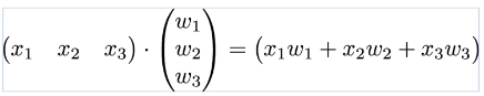
4. 행렬 연산을 고려하여 파이토치 구현
x_train  =  torch.FloatTensor([[73,  80,  75],
                               [93,  88,  93],
                               [89,  91,  80],
                               [96,  98,  100],
                               [73,  66,  70]])
y_train  =  torch.FloatTensor([[152],  [185],  [180],  [196],  [142]])
앞서 x_train을 3개 구현했던 것과 달리 x_train 안에 모든 샘플을 ( 5 * 3 ) 행렬로 선언한다.
# 가중치와 편향 선언
W = torch.zeros((3, 1), requires_grad=True)
b = torch.zeros(1, requires_grad=True)
여기서 중요한 점은 가중치 W가 크기 (3*1)벡터라는 것이다. 행렬의 곱셈이 성립되기 위해서 좌측에 있는 행렬의 열의 크기와 우측의 행렬의 행의 크기가 일치해야 한다. 현재 x_train이 (5*3)이고 W는 (3*1)이므로 두 행렬과 벡터는 행렬곱이 가능하다.
# optimizer 설정
optimizer = optim.SGD([W, b], lr=1e-5)

nb_epochs = 20
for epoch in range(nb_epochs + 1):

    # H(x) 계산
    # 편향 b는 브로드 캐스팅되어 각 샘플에 더해집니다.
    hypothesis = x_train.matmul(W) + b

    # cost 계산
    cost = torch.mean((hypothesis - y_train) ** 2)

    # cost로 H(x) 개선
    optimizer.zero_grad()
    cost.backward()
    optimizer.step()

    print('Epoch {:4d}/{} hypothesis: {} Cost: {:.6f}'.format(
        epoch, nb_epochs, hypothesis.squeeze().detach(), cost.item()
))'Background > Pytorch 기초' 카테고리의 다른 글
| 커스텀 데이터셋 (Custom Dataset) (0) | 2022.01.16 |
|---|---|
| 미니 배치와 데이터 로드 (Mini Batch and Data Load) (0) | 2022.01.16 |
| 클래스로 파이토치 선형회귀 모델 구현하기 (0) | 2022.01.14 |
| nn.Module로 구현하는 선형회귀 (0) | 2022.01.14 |
| 03-1 선형회귀(Linear Regression) (0) | 2022.01.14 |